Executive Summary

Transparency	Replicability	Clarity

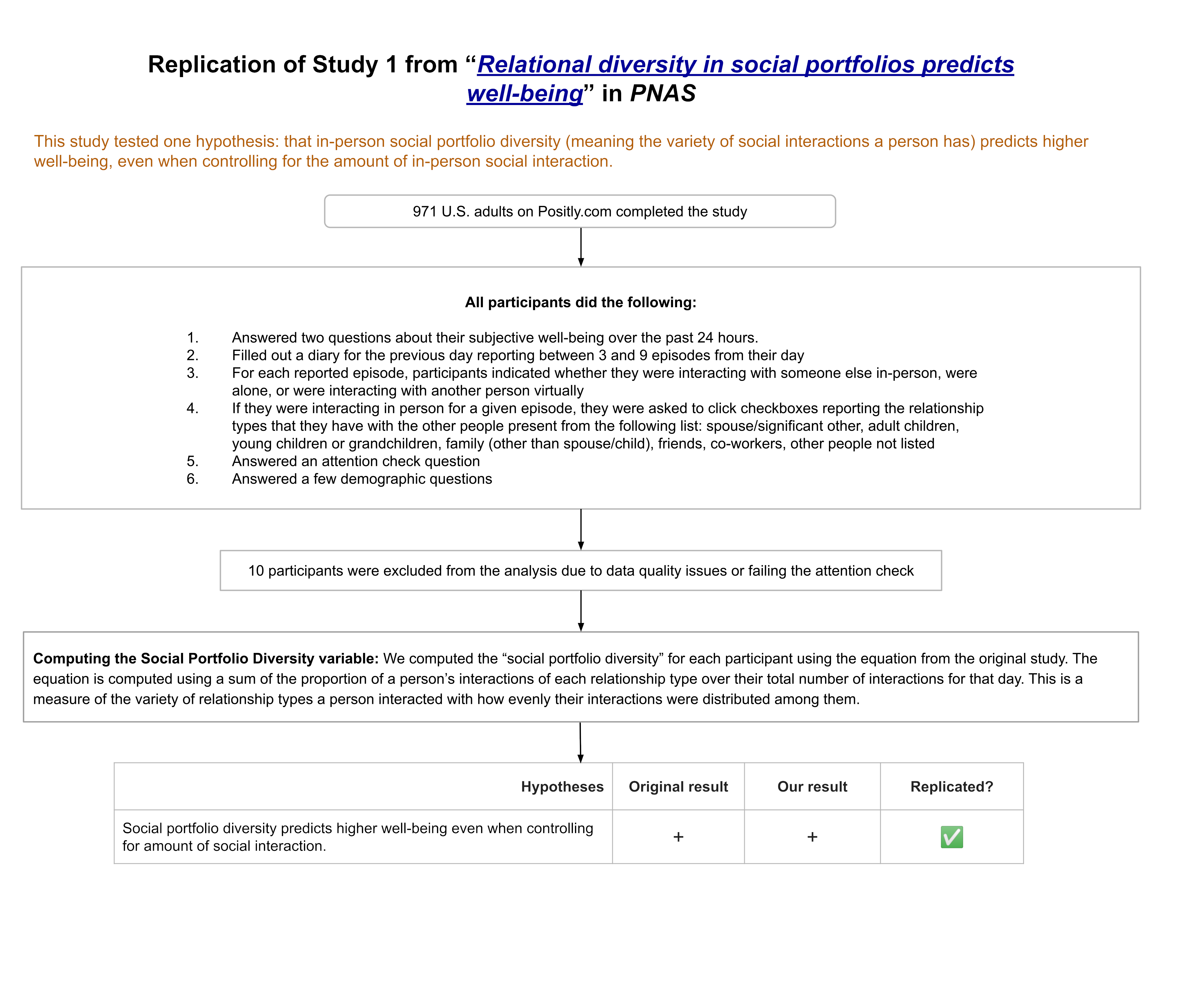
We ran a replication of study 1 from this paper, which found that the variety in a person’s social interactions predicts greater well-being, even when controlling for their amount of in-person social interaction.  This finding was replicated in our study. 

In this study participants were asked about their well-being over the last 24 hours, and then asked about their activities the previous day, including how many in-person interactions they had, and the kinds of relationships they have with the people in those interactions (e.g. spouse or partner, other family, friends, coworkers, etc.). The variety of interactions, called “social portfolio diversity,” had a positive association with well-being, above and beyond the positive effects due to the amount of social interaction.

Although this finding replicated, this paper has serious weaknesses in transparency and clarity. The pre-registered hypothesis differed from the hypothesis tested, and the authors do not acknowledge this in the paper. The main independent variable, social portfolio diversity, is described as being calculated in three conflicting ways in different parts of the paper and in the pre-registration. The findings reported in the paper are based on what we believe to be incorrect calculations of their primary independent and control variables (i.e., calculations that contradict the variable definitions given in the paper), and their paper misreports the sample size for their main analysis because the calculation error in the primary independent variable removed 76 cases from their analysis. Unfortunately, the authors did not respond to emails seeking clarification about their analysis.

Despite the flaws in the analysis, when these flaws were corrected, we found that we were indeed able to replicate the original claims of the paper – so the main hypothesis itself held up to scrutiny, despite inconsistencies and seeming mistakes with how calculations were performed.

(Update: On 8/9/2023 the authors wrote to us that they will be requesting that the journal update their article with a clarification.)

Full Report

Study Diagram

Replication Conducted

We ran a replication of Study 1 from: Collins, H.K., Hagerty, S.F., Quiodbach, J., Norton, M.I., & Brooks, A.W. (2022). Relational diversity in social portfolios predicts well-being. Proceedings of the National Academy of Sciences, 119(43), e2120668119. https://doi.org/10.1073/pnas.2120668119

How to cite this replication report: Transparent Replications by Clearer Thinking. (2023). Report #5: Replication of “Relational diversity in social portfolios predicts well-being” (PNAS | Collins et al. 2022) https://replications.clearerthinking.org/replication-2022pnas119-43

Key Links

• Our Research Box for this replication report includes the pre-registration, study materials, de-identified data, and analysis files.
• Manifold Markets predicted a 52% probability of this study replicating.
• Metaculus predicted a 62% probability of this study replicating.
• Download a PDF of the original paper.
• The supporting materials for the original paper can be found on OSF.

Overall Ratings

To what degree was the original study transparent, replicable, and clear?

Transparency:  how transparent was the original study?	This study provided data and experimental materials through OSF, which were strong points in its transparency. Analysis transparency was a weakness, as no analysis code was provided, and the authors did not respond to inquiries about a key analysis question that was left unanswered in the paper and supplemental materials. The study was pre-registered; however, the authors inaccurately claimed that their main hypothesis was pre-registered, when the pre-registered hypothesis did not include their control variable.
Replicability: to what extent were we able to replicate the findings of the original study?	The main finding of this study replicated when the control variable was calculated the way the authors described calculating it, but not when the control variable was calculated the way the authors actually did calculate it in the original paper. Despite this issue, we award the study 5 stars for replication because their key finding met the criteria for replication that we outlined in our pre-registration.
Clarity: how unlikely is it that the study will be misinterpreted?	Although the analysis used in this study is simple, and reasonable, there are several areas where the clarity in this study could be improved. The study does not report an R2 value for its regression analyses, which obscures the small amount of the variance in the dependent variable that is explained by their overall model and by their independent variable specifically. Additionally, the computation of the key independent variable is described inconsistently, and is conducted in a way that seems to be incorrect in an important respect. The sample size reported in the paper for the study is incorrect due to excluded cases based on the miscalculation of the key independent variable. The calculation of the control variable is not conducted the way it is described in the paper, and appears to be miscalculated. (Update: On 8/9/2023 the authors wrote to us that they will be requesting that the journal update their article with a clarification.)

Detailed Transparency Ratings

Overall Transparency Rating:
1. Methods Transparency:	A pdf showing the study as participants saw it was available on OSF.
2. Analysis Transparency:	Analysis code was not available and authors did not respond to emails asking questions about the analysis. A significant decision about how a variable is calculated was not clear from the paper, and we did not get an answer when we asked. Descriptions of how variables were calculated in the text of the paper and pre-registration were inconsistent with each other and inconsistent with what was actually done.
3. Data availability:	Data were available on OSF.
4. Pre-registration:	The study was pre-registered; however, the pre-registered hypothesis did not include the control variable that was used in the main analysis reported in the paper. The text of the paper stated that the pre-registered hypothesis included this control variable. The pre-registered uncontrolled analysis was also conducted by the authors, but the result was only reported in the supplementals and not the paper itself, and is not presented as a main result. Additionally, the pre-registration incorrectly describes the calculation method for the key independent variable.

Summary of Study and Results

Both the original study (N = 578) and our replication study (N = 961) examined whether the diversity of relationship types represented in someone’s in-person interactions in a given day predicts greater self-reported well-being the next day, beyond the effect of the total amount of in-person interaction in that day.

In the experiment, participants filled out a diary about their activities on the previous day, reporting 3 to 9 episodes from their day. For each episode they reported, participants were then asked about whether they were interacting with anyone in person, were interacting with anyone virtually, or were alone. For episodes where people reported in-person interactions, they were asked to check all of the checkboxes indicating the relationship types they had with the people in the interaction. The options were: spouse/significant other, adult children, young children or grandchildren, family (other than spouse/child), friends, co-workers, and other people not listed.

For each participant, we calculated their “social portfolio diversity” using the equation on p. 2 of the original study. More information about the computation of this variable is in the detailed results section. There were 971 participants who completed the study. We excluded 6 participants who failed the attention check from the data analysis, and 4 due to data quality issues, leaving N = 961. More details about the data exclusions is available in the appendix.

The dataset was analyzed using linear regression. The main analysis included social portfolio diversity as the main independent variable, the proportion of activities reported in the day that included in-person social interaction as a control variable, and the average of the two well-being questions as the dependent variable. The original study reported a statistically significant positive relationship between the social portfolio diversity variable and well-being in this analysis (β = 0.13, b = 0.54, 95% CI [0.15, 0.92], P = 0.007, n = 576), but please see the detailed results section for clarifications and corrections to these reported results. 

In our replication, we found that this result replicated both when the social portfolio diversity variable was calculated as 0 for subjects with no reported in-person interactions (β = 0.095, b = 0.410, 95% CI [0.085, 0.735], P = 0.014, n = 961) and when the 116 subjects with no in-person interactions reported are dropped due to calculating their social portfolio diversity as “NaN”  (β = 0.097, b = 0.407, 95% CI [0.089, 0.725], P = 0.012, n = 845). Note that calculating the control variable the way the original authors calculated it in their dataset, rather than the way they described it in the paper, resulted in non-significant results. Based on our pre-registered plan to calculate that variable the way it is described in the paper, we conclude that their main finding replicated. We are nonetheless concerned about the sensitivity of this finding to this small change in calculating the control variable.

Detailed Results

Computing the Social Portfolio Diversity and Amount of Social Interaction variables

(Update: On 8/9/2023 the authors wrote to us that they will be requesting that the journal update their article with a clarification.)

The “social portfolio diversity” equation is how the authors construct their primary independent variable. This equation involves computing, for each of the relationship categories a person reported having interactions with, the proportion of their total interactions that this category represented (which the authors call “p_i”). For each category of relationship, this proportion is multiplied by its natural logarithm. Finally, all these products are summed together and multiplied by negative one so the result is a positive number. The original authors chose this formula in order to make the “social portfolio diversity” variable resemble Shannon’s biodiversity index. 

How is p_i calculated in the Social Portfolio Diversity variable?

The computation of the “social portfolio diversity” variable is described by the authors  in three conflicting ways. From analyzing the data from their original study (as described in the section below on reproducing the original results), we were able to determine how this variable was actually calculated.

In the original paper the authors describe the calculation of the formula as follows:

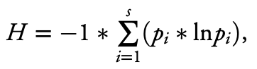
where s represents the total number of relationship categories (e.g., family member, coworker, close friend, stranger) an individual has reported interacting with, and p_i represents the proportion of total interactions (or proportion of total amount of time spent interacting) reported by a participant that falls into the ith relationship category (out of s total relationship categories reported). The diversity measure captures the number of relationship categories that an individual has interacted with (richness) as well as the relative abundance of interactions (or amount of time spent interacting) across the different relationship categories that make up an individual’s social portfolio (evenness) over a certain time period (e.g., yesterday). We multiply this value by -1, so higher portfolio diversity values represent a more diverse set of interaction partners across relationship categories (see Fig. 1).  [italicized and bolded for emphasis]

This description explains how the authors calculated the p_i variable. It’s important to note that here the “proportion of total interactions” is calculated by using the sum of the number of interaction types checked off for each episode, not the total number of episodes of in-person interaction. For example, if a person reported 3 episodes of their day with in-person interactions, and in all 3 they interacted with their spouse, and in 2 of those they also interacted with their kids, the p_i for spouse interactions is 3/5, because they had 3 spouse interactions out of 5 total interactions (the spouse interactions plus the child interactions), not 3 spouse interactions out of 3 total episodes with in-person interactions in the day. The description of how this variable is calculated in the “Materials and Methods” section of the paper describes this variable as being constructed using the second of these two methods rather than the first.  Here is that text from the paper:

Social portfolio diversity was calculated as follows: 1) dividing the number of episodes yesterday for which an individual reported interacting with someone in a specific social category by the total number of episodes they reported interacting with someone in any of the categories, giving us p_i; 2) multiplying this proportion by its natural log (p_i × ln p_i); 3) repeating this for each of the seven social categories; and 4) summing all of the (p_i × ln p_i) products and multiplying the total by -1. [italicized and bolded for emphasis]

In the pre-registration the calculation of this variable is described as:

From these questions, we will calculate our primary DV: Convodiversity

To calculate convodiversity, we will:

• Divide the number of times an individual interacted with someone in a certain social category in a day (e.g., spouse, friend, coworker) by the total number of people they interacted with that day, which gives us p_i.

• Multiply this proportion by its natural log (p_i X ln p_i).

• Repeat this for each specific social category assessed, and

• Sum all of the (p_i X ln p_i) products and multiple the total by -1.

This would be yet a third possible way of calculating p_i, which would result in 3 spouse interactions out of 2 people interacted with in the day for the example above.

It seems like the way that p_i was actually calculated is more likely to be both correct and consistent with the author’s intent than the other two possible ways they describe calculating p_i. We calculated Social Portfolio Diversity consistently with the way they actually calculated it for our analyses. Note that our experiment was coded to compute the Social Portfolio Diversity variable automatically during data collection, but this code was calculating the variable the way the authors described in the “Materials and Methods” section of their paper, prior to us noticing the inconsistency. We did not use this variable, and instead re-constructed the Social Portfolio Diversity variable consistently with the authors’ actual method.

How are people with no in-person episodes handled by the Social Portfolio Diversity equation?

The other problem we ran into in the calculation of the social portfolio diversity variable is what should be done when participants have 0 in-person social interactions reported for the day. Looking at the description of how the variable is calculated and the summation notation, it seems like in this case s, the total relationship categories reported, would be 0. This causes the equation to contain the empty sum, which resolves to 0, making the entire Social Portfolio Diversity equation for participants with no in-person social interactions resolve to 0.

That is not how the equation was resolved in the data analysis in the original paper. In the dataset released by the authors, the participants with no in-person social interactions reported for the day, have a value of “NaN” (meaning Not a Number) given for the Social Portfolio Diversity variable, and in the analyses that include that variable, these participants are excluded for having a missing value on this variable.

Because we did not hear back from the authors when we reached out to them about their intentions with this calculation, we decided to run the analysis with this variable computed both ways, and we pre-registered that plan.

How is the control variable calculated?

When we re-analyzed the authors’ original data, we used the perc_time_social variable that they included in their dataset as their control variable representing the total amount of in-person interaction in the day. Using that variable resulted in reproducing the authors’ reported results on their data; however, after doing that re-analysis, it later became clear that the “perc_time_social” variable that the authors computed was not computed the way they described in their paper. We were not aware of this issue at the time of filing our pre-registration, and we pre-registered that we would calculate this variable the way it was described in the paper, as “the proportion of episodes that participants spent socializing yesterday.” We interpreted this to mean the number of episodes involving in-person interactions out of the total number of episodes that the participant reported for their day. For example, imagine that a participant reported 9 total episodes for their day, and 7 of those episodes involved in-person interaction. This would result in a proportion of  7/9 for this variable, regardless of how many types of people were present at each episode involving in-person interaction.

When we examined the authors’ dataset more closely it became clear that their perc_time_social variable was not calculated that way. This variable was actually calculated by using the total number of interaction types for each episode added together, rather than the total episodes with in-person interaction, as the numerator. This is the same number that would be the denominator in the p_i calculation for the Social Portfolio Diversity variable. They then constructed the denominator by adding to that numerator 1 for each episode of the day that was reported that didn’t include in-person interactions. If we return to the example above, imagine that in the 7 episodes with in-person interaction, the participant reported interacting with their friends in 3, their spouse in 5, and their coworkers in 2. That would make the numerator of this proportion 10, and then for the denominator we’d add 2 for the two episodes with no in-person interaction, resulting in 10/12 as the proportion for this variable.

It is possible that this is what the authors actually intended for this variable, despite the description of it in the paper, because in the introduction to the paper they also describe this as controlling for the “total number of social interactions,” which could mean that they are thinking of this dyadically, rather than as episodes. This seems unlikely though, because calculating it this way incorporates aspects of social portfolio diversity into their control variable. It’s also a strange proportion to use because a single episode of in-person interaction could count for up to 7 in this equation, depending on the number of interaction types in them, while an episode without in-person interaction can only count as 1. The control variable seems intended to account for the amount of the day spent having in-person interactions, regardless of the particular people who were present. This is accomplished more simply and effectively by looking at the proportion of episodes, rather than incorporating the interaction types into this variable.

Despite this issue, these two methods of calculating this variable are highly correlated with each other (Pearson’s r = 0.96, p < .001 in their original data, and Pearson’s r = 0.989, p < .001 in our replication dataset). 

Reproducing the original results

Due to the original dataset evaluating participants with no reported in-person interactions as “NaN” for the Social Portfolio Diversity variable, it appears that the N the authors report for their Model 1 and Model 3 regressions is incorrect. They report an N of 577 for Model 1 and 576 for Model 3. The actual N for Models 1 and 3, with the cases with an “NaN” for Socal Portfolio Diversity excluded, is 500.

In their dataset of N = 578, their variable “ConvoDiv” (their Social Portfolio Diversity variable) is given as “NaN” in 78 cases. The regression results that are most consistent with the results they report are the results from N = 500 participants where “ConvoDiv” is reported as a number. If we modify their dataset and assign a 0 to the “ConvoDiv” variable for the 76 cases where a participant completed the survey but had no in-person social interaction the previous day, we get results that differ somewhat from their reported results. See the table below to see their reported results, and our two attempts to reproduce their results from their data. We attempted to clarify this by reaching out to the authors, but they did not respond to our inquiries.

	Reported results	Reproduced results	Reanalyzed results
	From Table S1 in the supplemental materials	Social Portfolio Diversity set to NA for people with no in-person episodes	Social Portfolio Diversity set to 0 for people with no in-person episodes
Model 1 Soc. Portfolio Div. only (IV only no control)	N = 577 Soc. Portfolio Div. β = 0.21, b = 0.84, 95%CI[0.50, 1.17] p < .001 R2 not reported	N = 500 Soc. Portfolio Div. β = 0.216, b = 0.835, 95%CI[0.504, 1.167] p < .001 R2 = 0.047 Adj. R2 = 0.045	N = 576 Soc. Portfolio Div. β = 0.241, b = 0.966, 95%CI[0.647, 1.285] p < .001 R2 = 0.058 Adj. R2 = 0.056
Model 3 Both Soc. Portfolio Div. (IV) and Prop. Inter. Social (control)	N = 576 Soc. Portfolio Div. β = 0.13, b = 0.54, 95%CI[0.15, 0.92] p = .007 Prop. Inter. Social β = 0.17, b = 0.99, 95%CI[0.32, 1.66] p = .004 R2 not reported	N = 500 Soc. Portfolio Div. β = 0.139, b = 0.537, 95%CI[0.150, 0.923] p = .007 Prop. Inter. Social β = 0.148, b = 0.992, 95%CI[0.321, 1.663] p = .004 R2 = 0.063 Adj. R2 = 0.059	N = 576 Soc. Portfolio Div. β = 0.133, b = 0.534, 95%CI[0.140, 0.927] p = .008 Prop. Inter. Social β = 0.180, b = 1.053, 95%CI[0.480,1.626] p < .001 R2 = 0.079 Adj. R2 = 0.076

Fortunately, the differences in the results between the two methods are small, and both methods result in a significant positive effect of Social Portfolio Diversity on well-being. We decided to analyze the data for our replication using both approaches to calculating the Social Portfolio Diversity variable because we wanted to both replicate exactly what the authors did to achieve the results they reported in their paper, and we also wanted to resolve the equation in the way we believe the authors intended to evaluate it (due to the equation they gave for social portfolio diversity and due to their reported N = 576). 

After determining that their calculation of the perc_time_social variable wasn’t as they described in the paper, and may not have been what they intended, we re-computed that variable as they described it, and re-ran their analyses on their data with that change (column 3 in the table below).

	Reported results	Reproduced results	Reanalyzed results
	From Table S1 in supplemental materials	using perc_time_social variable from original dataset	using proportion in-person episodes out of total episodes
Model 2 Control only	N = 576 Prop. Inter. Social β = 0.26, b = 1.53, 95%CI[1.07, 1.99] p < .001 R2 not reported	N = 577 perc_time_social β = 0.262, b = 1.528, 95%CI[1.068, 1.989] p < .001 R2 = 0.069 Adj. R2 = 0.067	N = 578 Prop. epi. In-person β = 0.241, b = 1.493, 95%CI[1.000, 1.985] p < .001 R2 = 0.058 Adj. R2 = 0.056
Model 3 IV & Control IV – NA for no interaction	N = 576 Soc. Portfolio Div. β = 0.13, b = 0.54, 95%CI[0.15, 0.92] p = .007 Prop. Inter. Social β = 0.17, b = 0.99, 95%CI[0.32, 1.66] p = .004 R2 not reported	N = 500 Soc. Portfolio Div. β = 0.139, b = 0.537, 95%CI[0.150, 0.923] p = .007 perc_time_social β = 0.148, b = 0.992, 95%CI[0.321, 1.663] p = .004 R2 = 0.063 Adj. R2 = 0.059	N = 500 Soc. Portfolio Div. β = 0.157, b = 0.606, 95%CI[0.234, 0.978] p = .001 Prop. ep. in-person β = 0.129 b = 0.89, 95%CI[0.223,1.558] p = .009 R2 = 0.060 Adj. R2 = 0.056
Model 3 IV & Control IV – 0 for no interaction		N = 576 Social Portfolio Div. β = 0.133, b = 0.534, 95%CI[0.140, 0.927] p = .008 perc_time_social β = 0.180, b = 1.053 95%CI[0.480,1.626] p < .001 R2 = 0.079 Adj. R2 = 0.076	N = 578 Social Portfolio Div. β = 0.152, b = 0.610, 95%CI[0.229, 0.990] p = .002 Prop. ep. In-person β = 0.157, b = 0.972, 95%CI[0.384,1.559] p = .001 R2 = 0.074 Adj. R2 = 0.071

We found that the coefficients for Social Portfolio Diversity are slightly stronger with the control variable calculated as the proportion of episodes reported that involve in-person interaction. In Model 2, using only the control variable, we found that when calculated as the proportion of episodes reported that involve in-person interaction the control variable explains slightly less of the variance than when it is calculated the way the authors calculated it. The R² for that model with the re-calculated control variable is 0.058. It was 0.069 using the perc_time_social variable as calculated by the authors.

We included the analysis files and data for these reanalyses in our Research Box for this report. The codebook for the data files marks variables that we constructed as “Added.” The other columns are from the dataset made available by the authors on OSF.

Our Replication Results

We  analyzed the replication data using both methods for calculating Social Portfolio Diversity, as discussed in our pre-registration. We also analyzed the data using both the way the control variable was described as being calculated (the way we said we would calculate it in our pre-registration), and the way the authors’ actually calculated it. We did this both ways because we wanted to conduct the study as we said we would in our pre-registration, which was consistent with how we believed the authors conducted it from the paper, and we also wanted to be able to compare their reported results to comparable results using the same variable calculations as the ones they actually did.

As with the original results, the two methods of calculating social portfolio diversity (dropping those people with no in-person social interactions or recording those participants as having a social portfolio diversity of zero) did not make a substantive difference in our results.

Unlike the original results, we found that there was a substantive difference in the results depending on how the control variable was calculated. When the control variable is calculated the way the authors calculated it in their original analyses, we find that the results do not replicate. When the control variable is calculated as the authors described in the paper (and how we pre-registered), we find that their results replicate. This difference held for both methods of calculating the social portfolio diversity variable. 

This was surprising given that the two versions of the control variable were correlated with each other at r = 0.989 in our data.  

Model 3 results using proportion of episodes as control variable

	Reanalyzed original results	Replication results
Model 3 IV & Control IV – NA for no interaction Control – Prop. episodes in-person	N = 500 Social Portfolio Div. β = 0.157, b = 0.606, 95%CI[0.234, 0.978] p = .001 Prop. ep. in-person β = 0.129, b = 0.89, 95%CI[0.223,1.558] p = .009 R2 = 0.060 Adj. R2 = 0.056	N = 845 Social Portfolio Div. β = 0.097, b = 0.407, 95%CI[0.089, 0.725] p = .012 Prop. ep. in-person β = 0.228, b = 1.556, 95%CI[1.042, 2.070] p < .001 R2 = 0.084 Adj. R2 = 0.082	✅
Model 3 IV & Control IV – 0 for no interaction Control – Prop. episodes in-person	N = 578 Social Portfolio Div. β = 0.152, b = 0.610, 95%CI[0.229, 0.990] p = .002 Prop. ep. in-person β = 0.157, b = 0.972, 95%CI[0.384,1.559] p = .001 R2 = 0.074 Adj. R2 = 0.071	N = 961 Social Portfolio Div. β = 0.095, b = 0.410, 95%CI[0.085, 0.725] p = .014 Prop. ep. in-person β = 0.263, b = 1.617, 95%CI[1.154, 2.080] p < .001 R2 = 0.108 Adj. R2 = 0.106	✅

Model 3 results using proportion of interactions as in original analysis as control variable

	Reanalyzed original results	Replication results
Model 3 IV & Control IV – NA for no interaction Control – perc_time _social as in original paper	N = 500 Social Portfolio Div. β = 0.139, b = 0.537, 95%CI[0.150, 0.923] p = .007 perc_time_social β = 0.148, b = 0.992, 95%CI[0.321, 1.663] p = .004 R2 = 0.063 Adj. R2 = 0.059	N = 845 Social Portfolio Div. β = 0.057, b = 0.242, 95%CI[-0.102, 0.586] p = .168 propSocialAsInOrigPaper β = 0.256, b = 1.691, 95%CI[1.151,2.231] p < .001 R2 = 0.087 Adj. R2 = 0.085	❌
Model 3 IV & Control IV – 0 for no interaction Control – perc_time _social as in original paper	N = 576 Social Portfolio Div. β = 0.133, b = 0.534, 95%CI[0.140, 0.927] p = .008 perc_time_social β = 0.180, b = 1.053, 95%CI[0.480,1.626] p < .001 R2 = 0.079 Adj. R2 = 0.076	N = 961 Social Portfolio Div. β = 0.055, b = 0.240, 95%CI[-0.112, 0.592], p = .182 propSocialAsInOrigPaper β = 0.292, b = 1.724, 95%CI[1.244, 2.205],  p < .001 R2 = 0.111 Adj. R2 = 0.109	❌

Due to the fact that we pre-registered calculating the control variable as “the number of episodes that involved in-person interaction over the total number of episodes the participant reported on,” and that we believe that this is a more sound method for calculating this variable, and it is consistent with how the authors described the variable in the text of their paper, we consider the main finding of this paper to have replicated, despite the fact that this is not the case if the control variable is calculated the way the authors actually calculated it in their reported results. Results for the Model 1 and Model 2 regressions are available in the appendix, as they were not the main findings on which replication of this study was evaluated.

Interpreting the Results

Despite the fact that these results replicated, we would urge caution in the interpretation of the results of this study. It is concerning that a small change in the calculation of the control variable to the method actually used by the authors in their original data analysis is enough to make the main finding no longer replicate. Additionally, the change in model R² accounted for by the addition of the social portfolio diversity variable to a model containing the control variable is very small (in our replication data the change in R² is 0.006 or 0.007 depending on how the social portfolio diversity variable is calculated). As mentioned earlier, the authors did not report the model R² anywhere in their paper or supplementary materials. 

Conclusion

The errors and inconsistencies in the computation and reporting of the results were a major concern for us in evaluating this study, and resulted in a low clarity rating, despite the simplicity and appropriateness of the analysis that was described in the paper. The claim in the paper that the main hypothesis was pre-registered, when the pre-registered hypothesis was different than what was reported in the paper, and the lack of response from the authors to emails requesting clarification about their social portfolio diversity variable, reduced the transparency rating we were able to give this study, despite the publicly accessible experimental materials and data. Despite these issues, we did find that the main finding replicated. 

(Update: On 8/9/2023 the authors wrote to us that they will be requesting that the journal update their article with a clarification.)

Acknowledgements

We are grateful to the authors for making their study materials and data available so that this replication could be conducted.

We provided a draft copy of this report to the authors for review on June 22, 2023. 

Thank you to Clare Harris at Transparent Replications who provided valuable feedback on this replication and report throughout the process. We appreciate the people who made predictions about the results of this study on Manifold Markets and on Metaculus. Thank you to the Ethics Evaluator for their review, and to the participants for their time and attention.

Purpose of Transparent Replications by Clearer Thinking

Transparent Replications conducts replications and evaluates the transparency of randomly-selected, recently-published psychology papers in prestigious journals, with the overall aim of rewarding best practices and shifting incentives in social science toward more replicable research.

We welcome reader feedback on this report, and input on this project overall.

Appendices

Additional Information about the Methods

Exclusion Criteria

We collected 971 complete responses to this study, and analyzed data from 961 subjects. The following table explains our data inclusion and exclusion choices.

Category	Number of Subjects	Excluded or Included	Reason
Attention Check	6	Excluded	Responded incorrectly to the attention check question by checking boxes other than “None of the above”
Attention Check	7	Included	Did not check any boxes in response to the attention check question. One subject reported in feedback on the study that they were not sure if they were supposed to select the option labeled “None of the above” for the attention check, or not select any of the checkboxes. Reanalyzing the data with these 7 subjects excluded does not change the results in any substantive way. These subjects are marked with a 1 in the column labeled AttnCheckLeftBlank.
Data Quality	2	Excluded	A visual inspection of the diary entries revealed two subjects who entered random numbers for their episode descriptions, and spent less than 2 minutes completing the study. All other subjects provided episode descriptions in words that were prima facia plausible. These two subjects were excluded due to a high likelihood that their responses were low quality, despite them passing the attention check question.
Data Quality	2	Excluded	Due to inconsistencies created when subjects edited diary entries, 2 subjects reported more than 9 episodes for the day. Reducing those episodes to the maximum of 9 would have required making decisions about whether to eliminate episodes involving in-person interaction or episodes not involving interaction, which would have impacted the results, therefore these two subjects’ responses were excluded.
Data Quality	10	Included	Due to inconsistencies created when subjects entered or edited their diary entries, 10 subjects’ numbers reported for total episodes or for in-person episodes were incorrect. These subjects’ data were able to be corrected using the saved diary information, without the need to make judgment calls that would impact the results, therefore these subjects’ data were included in the analysis. Reanalyzing the data with these 10 subjects excluded does not change the results in any substantive way. These subjects are marked with a 1 in the column labeled Corrected.

Additional information about the results

Model 1 results comparing original data and replication data

	Reanalyzed Original Results	Replication Results
Model 1 IV only IV – NA for no interaction	N = 500 Social Portfolio Div. β = 0.216, b = 0.835, 95%CI[0.504, 1.167] p < .001 R2 = 0.047 Adj. R2 = 0.045	N = 845 Social Portfolio Div. β = 0.214, b = 0.901, 95%CI[0.623, 1.179] p < .001 R2 = 0.046 Adj. R2 = 0.045	✅
Model 1 IV only IV – 0 for no interaction	N = 576 Social Portfolio Div. β = 0.241, b = 0.966, 95%CI[0.647, 1.285] p < .001 R2 = 0.058 Adj. R2 = 0.056	N = 962 Social Portfolio Div. β = 0.254, b = 1.098, 95%CI[0.833, 1.363] p < .001 R2 = 0.064 Adj. R2 = 0.063	✅

Model 2 results comparing original data and replication data

	Reanalyzed Original Results	Replication Results
Model 2 Control only Control – perc_time _social as in original paper	N = 577 perc_time_social β = 0.262, b = 1.528, 95%CI[1.068, 1.989] p < .001 R2 = 0.069 Adj. R2 = 0.067	N = 961 propSocialAsInOrigPaper β = 0.330, b = 1.946, 95%CI[1.593, 2.299] p < .001 R2 = 0.109 Adj. R2 = 0.108	✅
Model 2 Control only Control – Prop. episodes in-person	N = 578 Prop. ep. in-person β = 0.241, b = 1.493, 95%CI[1.000, 1.985] p < .001 R2 = 0.058 Adj. R2 = 0.056	N = 961 propInPersonEpisodes β = 0.320, b = 1.970, 95%CI[1.601, 2.339] p < .001 R2 = 0.103 Adj. R2 = 0.102	✅

References

Collins, H.K., Hagerty, S.F., Quiodbach, J., Norton, M.I., & Brooks, A.W. (2022). Relational diversity in social portfolios predicts well-being. Proceedings of the National Academy of Sciences, 119(43), e2120668119. https://doi.org/10.1073/pnas.2120668119 

Faul, F., Erdfelder, E., Buchner, A., & Lang, A.-G. (2009). Statistical power analyses using G*Power 3.1: Tests for correlation and regression analyses. Behavior Research Methods, 41, 1149-1160. Download PDF